• Menu
  • Skip to right header navigation
  • Skip to main content

Ultracold Fermi Gases @ Technion

Prof. Yoav Sagi's Lab

  • Welcome
  • Research
  • Our System
  • People
  • Publications
  • Talks & Media Resources
  • Contact
  • Welcome
  • Research
  • Our System
  • People
  • Publications
  • Talks & Media Resources
  • Contact

Shortcut to adiabaticity

.[latexpage]

Read more in our publication:

  • Ness, G., Shkedrov, C., Florshaim, Y., Sagi., Y. Realistic Shortcuts to Adiabaticity in Optical Transfer, New J. Phys. 20, 095002 (2018).

The question we ask is how to perform dynamical changes as fast as possible without causing heating? the prime example we focus on is optical transport of ultracold atoms between two locations.

Why non-adiabatic transport? True adiabaticity takes asymptotically long time which leads to decoherence, noise and overall slower repetition rate.

The solution: Shortcuts to Adiabaticity (STA).

Shortcuts to adiabaticity refers to a class of schemes enabling the fast variation of a system Hamiltonian while still reaching a specific target state. They derived by cleverly tailoring the fast driving protocol such that the system attains the desired final state without being adiabatic. However, the experimental implementation of STA for rapid atoms transfer suffers from an inherent problem arising from the fact that these driving profiles are suited for the atoms trajectory as in practice the trap coordinate is the controlled one. In our research, the experimental realization of these STA schemes was achieved for optical transfer of ultracold fermionic atoms. We found that in order to lift conflicting boundary conditions it is necessary to increase the number of degrees of freedom in the trajectory, develop and demonstrate two complementary methods to achieve this; the first acts as a “correction” to the original trajectory, while in the second approach the trajectory is redesigned to account for all boundary conditions. Using both methods, we demonstrate successful transports of cold atoms in the highly non-adiabatic regime.

Method 1: Spectral correction

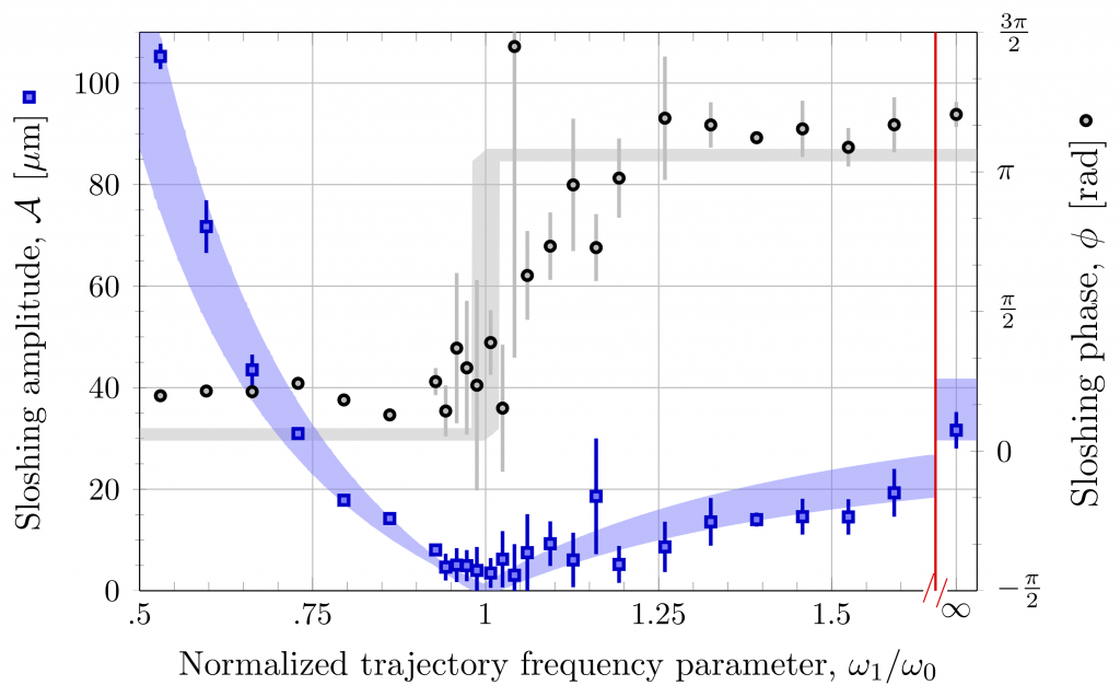
Approximating the optical potential to a harmonic one, the requirement for STA transport reduces to zero sloshing amplitude at transport end. The terminate sloshing amplitude can be analytically calculated by the trapping frequency Fourier component of the trap velocity trajectory,

$\mathcal{A}\left(t_{f}\right)
=\left|\intop_{0}^{t_{f}}\exp\left(-i\omega_{0}t\right)\dot{z}_{\cup}\left(t\right)\mathrm{d}t\right|$.

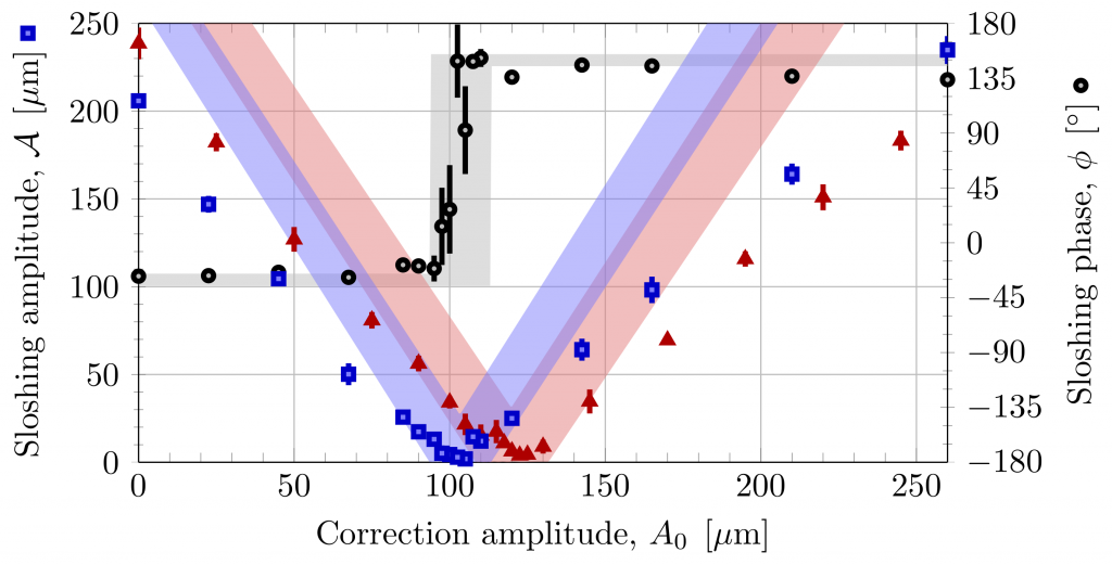
The idea in this method is to introduce a new spectral component to an existing trajectory which can be implemented experimentally such that it will satisfy all required boundary conditions and the sloshing amplitude will vanish. We can cancel the sloshing amplitude by adding a new spectral component at the trapping frequency such that their sum is zero. A scan of the correction amplitude at the optimal correction phase is presented in Fig.1

Fig1.: Sloshing mode amplitude (blue squares) and phase (gray circles) versus the spectral correction amplitude, after non-adiabatic movement with polynomial trajectory. Theoretical harmonic calculations appear as ribbons with matching colors, where the width is determined by the trapping frequency uncertainty. These measurements were performed following transport of $d=1.29\thinspace\mathrm{mm}$ lasting $t_{f}=186\thinspace\mathrm{ms}$ in a trap of axial frequency $\omega_{0}=2\pi\cdot7.16\left(15\right)\thinspace\mathrm{Hz}$ ($f_{0}\cdot t_{f}=1.33\left(3\right)$). The motion of warmer atomic ensembles was also corrected. The red triangles indicate the sloshing amplitudes of the same trajectories but for atoms that were pre-warmed before the experiment. As the temperature increases, the atoms experience more the non-harmonic terms and the effective harmonic trapping frequency decreases. The temperature and number of atoms are $T=320\left(30\right)\thinspace\mathrm{nK}$ and $N=390(20)\cdot {10}^{3}$ for the blue squares, and $T=510\left(70\right)\thinspace\mathrm{nK}$ and $N=380(20)\cdot {10}^{3}$ for the red triangles. The frequency shift for the red ribbon was calculated according to the measured extent of both atomic clouds in the trap before the motion with no fitting parameter.
 
Even in the anharmonic case, it is still true that the sloshing mode is the first to be excited from a rapid shift of the trap. Hence, nullifying the sloshing amplitude will provide us with a trajectory very close to optimum. The anharmonicity can be incorporated into an effective harmonic frequency by virtue of the fermionic energy distribution. In the case of a Gaussian beam, the frequency decreases with increasing temperature, an effect referred to as “softening”. To study how anharmonicity affects the STA, we repeated the experiments of Fig.\,\ref{fig1} with temperature increased by $\times1.6$ using parametric excitation. The axial \emph{in situ} variance of the atomic cloud density $\left\langle\left(z-z_\cup\right)^{2}\right\rangle$ before the transport is about $\left(229\thinspace\mathrm{\mu m}\right)^2$ and $\left(272\thinspace\mathrm{\mu m}\right)^2$ for the cold and hot clouds, respectively. A good estimate for the radial variance $\left\langle r^{2} \right\rangle$ can be obtained using the known aspect ratio of the trapping frequencies in the axial and radial directions. Using this data we calculate the ratio between the effective harmonic frequencies in the two experimental conditions and obtain $\frac{\omega^{\prime}_{\mathrm{cold}}}{\omega^{\prime}_{\mathrm{hot}}}=1.027$. For this, we can numerically find a new optimum value for correction amplitude $A_0$. The correction phase $\phi_0$, however, is unaffected by this variation of the effective frequency. 

Method 2: Spectral correction

In the second method, in order to comply with all of the eight boundary conditions, we use a polynomial trajectory of the seventh order. This path for the atoms respects the invariant necessitated boundary conditions and its associated trap trajectory results with zero velocities at motion ends, so it is feasible to be implemented experimentally.
The desirable path of the trap is dependent the trapping frequency $\omega_{0}$, so one is required to provide the later with great accuracy in order to respect the boundary conditions and accomplish the transport with zero sloshing amplitude. In Fig.2 we present the sloshing amplitudes following such a trajectory where we scan the value of the frequency parameter. Indeed, for the correct value of the frequency parameter, we observe a sloshing amplitude consistent with zero. The right-hand side data points are in fact the case where we used the trajectory $z_{7}\left(t\right)$ directly for the trap itself, which results in a considerable excess energy.
 
Fig.2.: Non-adiabatic transfer with a septic polynomial trajectory. Plotted are the sloshing amplitude (blue squares) and phase (gray circles) following a septic trajectory: $z_{\cup}\left(t\right)=z_{7}\left(t\right)+\ddot{z}_{7}\left(t\right)/\omega_{1}^{2}$ versus the frequency parameter $\omega_1$. Theoretical harmonic calculations appear as ribbons with matching colors, where the width is determined by the frequency uncertainty. Minimum sloshing consistent with zero appears in the vicinity of the real oscillation frequency $\omega_1=\omega_0$. The sloshing measurements performed following a $1.29\thinspace\mathrm{mm}$ transport during $t_{f}=273\thinspace\mathrm{ms}$ in a trap of axial frequency $\omega_{0}=2\pi\cdot7.55\left(8\right)\thinspace\mathrm{Hz}$ ($f_{0}\cdot t_{f}\approx2$).
 

Copyright © 2025 · Prof. Yoav Sagi · yoav.sagi@physics.technion.ac.il
Developed and maintained by the Web Development Group, Physics Department, Technion